Feedforward propagation - A Simple Introduction to neural networks

Neural Networks

A neural network is many neurons interconnected with each other. Each neuron performs small and simple functions but in aggregation, they do some very useful tasks. They are based on how human brains work, and their fundamental task is to recognize patterns.

Feedforward Neural Network

Feedforward Neural Network is the simplest neural network. It is called Feedforward because information flows forward from Inputs -> hidden layers -> outputs. There are no feedback connections. The model feeds every output to the next layers and keeps moving forward.

There is another type of neural network where the output of the model is fed to itself is called recurrent neural networks.

figure 1. Architecture of neural network

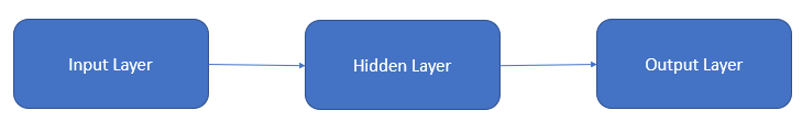
This is a higher-level architecture of a single neural network. The input layer contains our input data which have information to predict the output. Data gets manipulated and different mathematical operations take place when it travels through hidden layers and to the output. The output provides the predicted value. Each layer has several neurons which are called units.

figure 2. Simple neural network

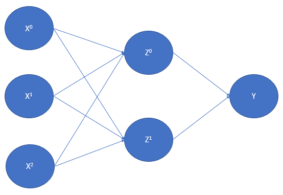
This is an example of a simple feedforward neural network. The leftmost layer is the input layer, the middle layer is the hidden layer and last is the output layer. It is a single layer hidden layer network with 2 hidden units. Hidden layers and units can be increased based on the requirements.

Dataset

We take a small dataset as an example. The dataset contains information about candidates who applied for a job and we also have data of their job offer results i.e. they got a job offer or not.

table 1. Given data

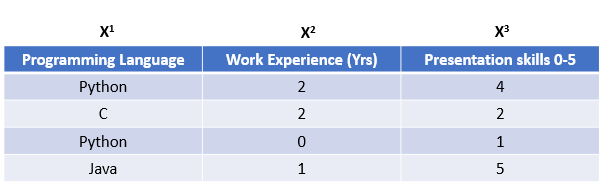
Here X1, X2, and X3 are called features. In Machine Learning, there needs to be a balance of the number of features as more features would lead to overfitting and fewer features would lead to underfitting.

table 2. True value of given data

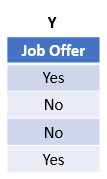
This is the result of the candidates. 1st and 4th got an offer and others did not. So now using this dataset, we want to predict if a new candidate has certain skills, will he get a job offer or not. Hence this data that we have is the training data.

Algorithm

figure 3. Feedforward propagation on single layer network

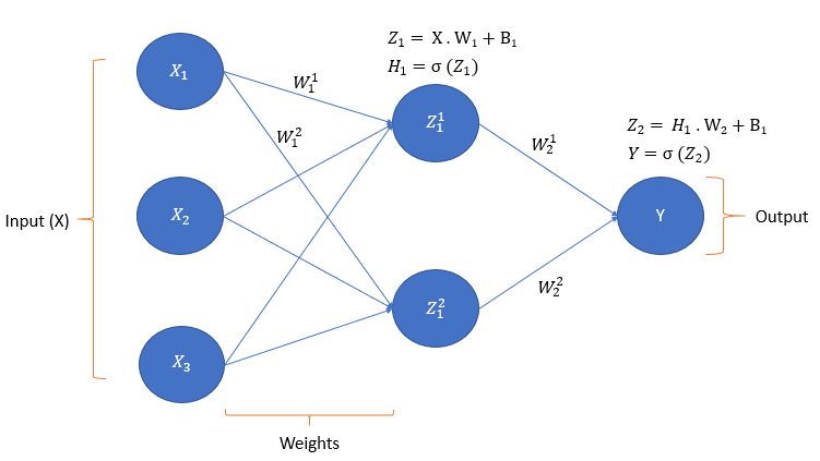
This image shows the working of a simple feedforward neural network.

Notations

Working of the network

Generally, weights are initialized with random weights between \( (0,1) \) or \( (-1,1) \). You can initialize it with any other value. The initial value of \(W\) may affect the result or other parameters like the required number of iterations. Weights are created to maintain how much proportion of each feature of the dataset is important for prediction. Weights are assigned values accordingly. We shall discuss this further after the algorithm. Same way bias is generally initialized with all \(1\) values.

After we get the value of \(Z_1\), we pass it to the activation function. There are many different activation functions whose purpose is to decide whether a neuron or a unit should be activated or not. It's also used to introduce non-linearity to the output of the neuron. We will take sigmoid as an activation function. Its formula is \( \frac{e^x}{(1 + e^{-x})} \). Hence \( \sigma (Z_1) \) gives us a result of the sigmoid function i.e. \( H_1 = \sigma (Z_1) \).

As you can see, we calculated \(Z_2\) taking \(H_1\) as the input of the output layer i.e \(H_1\) becomes \(X\) here. The shape of \(H_1\) is \(4 \times 2\) and \(W_2\) is \(2 \times 1\). \(B_2\) is now \(1 \times 1\). Then we pass \(Z_2\) to the sigmoid function to get \(Y\) which is the predicted output of our network. This is the full working of the feedforward network. As our network has only one neuron in the output layer, the output vector would be \((4 \times 1)\).

2 layer network

As we saw feedforward propagation on single layer network, now lets see the algorithm for 2 layer network. This will give you better idea on how the network can be expanded and calculated.

figure 4. Feedforward propagation on 2 layer network

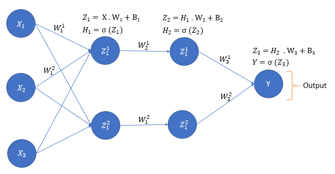
$$ Z_1 = X \cdot W_1 + B_1 $$

$$ H_1 = \sigma(Z_1) $$

$$ Z_2 = H_1 \cdot W_2 + B_2 $$

$$ H_2 = \sigma(Z_2) $$

$$ Z_3 = H_2 \cdot W_3 + B_3 $$

$$ Y = \sigma(Z_3) $$

Loss

After training the network we test our network using testing data and its labels(true output). We test it based on its error rate % or loss. There are different types of loss functions. One of them is mean square error which is:

Where \(Y\) is the output of the network (predicted value) and \(T\) is the true value of the data.

Conclusion

As mentioned earlier, weights are used to maintain how much priority to give to each feature and how much proportion of each feature takes part in the prediction. As we have initialized weights with random values, which are not ideal and do not know which features are of how much importance. We need to set our weights value based on this requirement. We do not know the value of ideal weights, for which we use an algorithm call backpropagation. It propagates from backward and updates weights on every iteration based on loss of the network.

During training, All these calculations happen for \(N\) number of iterations. In each iteration, \(Y\) is calculated using feedforward, a loss is calculated, and backpropagation updates the weights. In the next iteration, everything is calculated based on the updated weights. Hence weights keep updating in each iteration leading to better accuracy for prediction.