Backpropagation - A pillar of neural networks
April 22, 2020
Harsh Patel
Hello people, this blog is about the backpropagation algorithm used in Machine learning. It is one of the most important algorithms and can be described as the pillar of the neural networks. I tried to make it as simple as possible, so I am sure you would be able to understand the fundamental working of backpropagation after reading this blog.
Overview
As we have seen in the last post that during training, Neural networks undergo feedforward and backpropagation mechanism. Data moves from input to output i.e. first layer to the last layer in feedforward mechanism and then we start backward and move from right to left to again first layer in backpropagation. The main purpose of backpropagation is that we update other parameters of the network with a change in a loss.
Introduction
From input data, we generate predicted data using feedforward propagation. then we find a loss between predicted data and true data. Now as loss gets updated, we need to update all network parameters before the next iteration. So, using backpropagation, we update all the values for the change in a loss. We use chain rule in derivation to calculate this.
Feedforward at a glance
Notations:
$$ T = \text{true data} $$ $$ L = loss $$ $$ Y = \text{predicted data} $$ $$ W = \text{weights ( }W_1 \text{ means layer 1 weights) } $$ $$X = \text{input data} $$ $$B = bias $$
$$ Z_1 = X \cdot W_1 + B_1 $$
$$ H_1 = \sigma(Z_1) $$
$$ Z_2 = H_1 \cdot W_2 + B_2 $$
$$ Y = \sigma(Z_2) $$
$$ L = \frac{1}{N} \sum_{i=0}^{N} (Y-T)^{2} $$
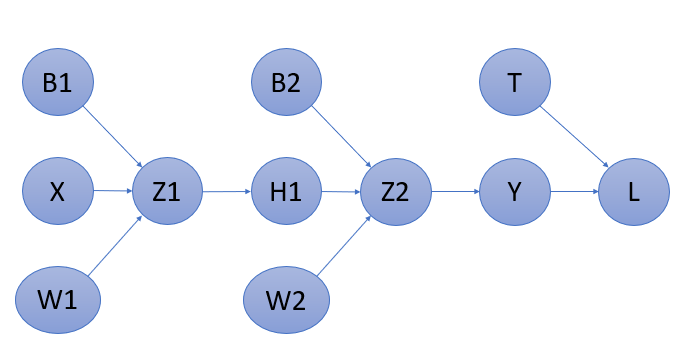
The above computation graph shows single hidden layer working of the network. If you are not able to understand it, you can know more about the feedforward network on my previous blog. click here.
Backpropagation
Backpropagation is calculated for \(n+1\) times for \(n\) layer network. In other words, No. of backpropagation = No. of weights in the network so there will be 2 times backpropagation according to above network.
Now Let’s look at backpropagation for \(W_2\) (last weight) in the network. As we have discussed before, we have to find the change of other values with change in loss.
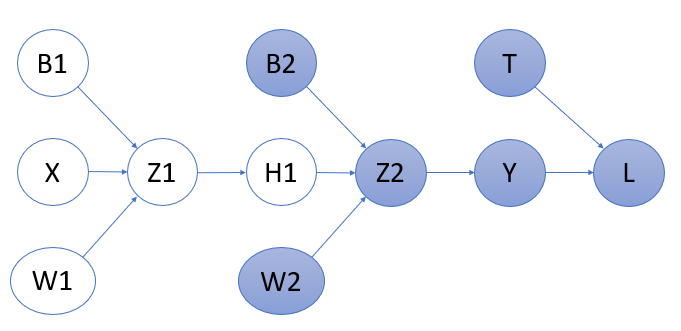
Last layer backpropagation includes all the highlighted circles as shown in the above figure 2. So the values we need to find are:
$$ \frac{\partial L}{\partial Y} = \text {change of Y with loss} $$ $$ \frac{\partial Y}{\partial Z_2} = \text {change of Z with Y} $$ $$ \frac{\partial Z_2}{\partial W_2} = \text {change of W with Z} $$ $$ \frac{\partial Z_2}{\partial B_2} = \text {change of B with Z} $$
$$ \frac{\partial L}{\partial Y} , \frac{\partial Y}{\partial Z_2} , \frac{\partial Z_2}{\partial W_2} , \frac{\partial Z_2}{\partial B_2} $$
Of course, we can find all these values, but here is a question, what values can we update after calculating them? We cannot update \(Y\) or \(Z\) as it is generated by the model. We can change bias and weights as we initialize it from the start. Bias and weights does gets manipulated throughout the layers. Weights decide how many features should be propagated further. We can also not change input data as changing it will not be a good idea ever (we want to find a solution to the problem, not change the problem). So we are going to update only these values.
$$ \frac{\partial Z_2}{\partial W_2} , \frac{\partial Z_2}{\partial B_2} $$
To compute this, we will apply the chain rule. Chain rule works as follows:
$$ \frac{\partial a}{\partial d} = \frac{\partial a}{\partial b} \times \frac{\partial b}{\partial c} \times \frac{\partial c}{\partial d} $$
Hence applying it in our scenario:
$$ \frac{\partial L}{\partial W_2} = \frac{\partial L}{\partial Y} \times \frac{\partial Y}{\partial Z_2} \times \frac{\partial Z_2}{\partial W_2} \quad,\quad \frac{\partial L}{\partial B_2} = \frac{\partial L}{\partial Y} \times \frac{\partial Y}{\partial Z_2} \times \frac{\partial Z_2}{\partial B_2}$$
An example
This is like passing a message to each node backward. Let us take a small example to understand this better. Suppose you are going on a trip to Las Vegas with a budget of 30K. Now you want to know how much money you will be left with for using in casino eliminating other expenses. You have an idea that 10% will be travel cost and 20% will be accommodation cost.
Let us compute this problem and help you out with it.
Budget = 30K
travel cost = 30K * 0.10 = 3K
accommodation cost = 30K * 0.20 = 6K
Money after eliminating costs = 21K
Hence you will have 21K to use In the casino. Now if you change the budget, you would have to compute all the costs again to calculate remaining money.
Same way as you find loss, you need to change all the intermediate values which finally gives you the changes in weights and bias. This would have given you an idea of why and what happens.
Continuing further
Now let us calculate chain rule derivatives.
\( \text{Sigmoid as an activation function } \sigma = \frac{e^x}{(1 + e^{-x})} \)
\( \text{derivative of sigmoid } \sigma = \sigma' = \sigma(x) \times (1 - \sigma(x)) \)
\( \text{MSE loss } = \frac{1}{N} \sum_{i=0}^{N} (y-t)^{2} \)
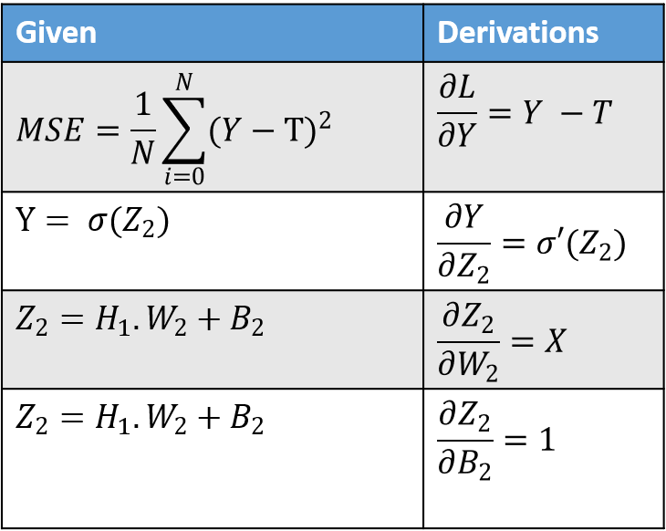
Using table 1. we get the following values.
$$ \frac{\partial L}{\partial W_2} = (Y - T) \times \sigma'(Z_2) \times X $$ $$ \text{As } \frac{\partial Z_2}{\partial B_2} = 1, \quad \frac{\partial L}{\partial B_2} = (Y - T) \times \sigma'(Z_2) \quad \text{i.e. equal to }\ \frac{\partial L}{\partial Z_2} $$
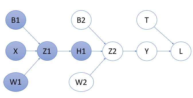
We completed \(1\) backpropagation , we will now move further and calculate for \(W_1\) (i.e. the first weight of our network) and then generate a formula for the arbitrary number of layers.
Till now, we have computed
$$ \frac{\partial L}{\partial Z_2} = (Y - T) \times \sigma'(Z_2) $$ $$ \frac{\partial L}{\partial W_2} = (Y - T) \times \sigma'(Z_2) \times X $$
Applying Chainrule for \(2^{nd} \) backpropagation :-
$$ \frac{\partial L}{\partial W_1} = \frac{\partial L}{\partial Y} \times \frac{\partial Y}{\partial Z_2} \times \frac{\partial Z_2}{\partial H_1} \times \frac{\partial H_1}{\partial Z_1} \times \frac{\partial Z_1}{\partial W_1} $$ $$ \frac{\partial L}{\partial B_1} = \frac{\partial L}{\partial Y} \times \frac{\partial Y}{\partial Z_2} \times \frac{\partial Z_2}{\partial H_1} \times \frac{\partial H_1}{\partial Z_1} \times \frac{\partial Z_1}{\partial B_1} $$Because we already know \( \frac{\partial L}{\partial Z_2} \)from previous calculations, we can simplify this as,
$$ \frac{\partial L}{\partial W_1} = \frac{\partial L}{\partial Z2} \times \frac{\partial Z_2}{\partial H_1} \times \frac{\partial H_1}{\partial Z_1} \times \frac{\partial Z_1}{\partial W_1} $$ $$ \frac{\partial L}{\partial B_1} = \frac{\partial L}{\partial Z2} \times \frac{\partial Z_2}{\partial H_1} \times \frac{\partial H_1}{\partial Z_1} \times \frac{\partial Z_1}{\partial B_1} $$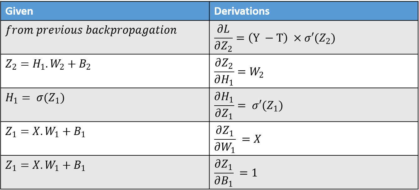
Using table 2. we get the following values.
$$ \frac{\partial L}{\partial W_1} = \frac{\partial L}{\partial Z_2} \times W_2 \times \sigma'(Z_1) \times X $$ $$ \frac{\partial L}{\partial B_1} = \frac{\partial L}{\partial Z_2} \times W_2 \times \sigma'(Z_1) \times 1 $$
expanding we get,
$$ \frac{\partial L}{\partial W_1} = (Y - T) \times \sigma'(Z_2) \times W_2 \times \sigma'(Z_1) \times X $$ $$ \frac{\partial L}{\partial B_1} = (Y - T) \times \sigma'(Z_2) \times W_2 \times \sigma'(Z_1) \times 1 $$
So, we calculated all required derivatives required for backpropagation for a single layer neural network.
Arbitrary number of layers
We can observe that each time we calculate backpropagation, we already have some values of the previous calculations in the chainrule. So we can and keep multiplying further with those values as we go on. we notice that in both \( \frac{\partial L}{\partial W_1}\) and \(\frac{\partial L}{\partial W_2}\), we have some common values. The common values are :
$$ (Y - T) \times \sigma'(Z_2) \times X $$
and what gets added in second backpropagation is :
$$ W_2 \times \sigma'(Z_1) $$
When we also calculate for 3rd backpropagation in a more dense network, we find out that each time this same values keeps adding up for each layer and the common value remains fixed. Using this observations we derive a general formula for any network as the following.
$$ n = \text{total hidden layers of network} + 1 = \text{total weights of the network} $$
$$ \frac{\partial L}{\partial B_k} = (Y - T) \times \sigma'(Z_n) \times \prod_{i=2}^{k} {W_{k} \times \sigma'(Z_{k-1})} $$ $$ \frac{\partial L}{\partial W_k} = (Y - T) \times \sigma'(Z_n) \times X \times \prod_{i=2}^{k} {W_{k} \times \sigma'(Z_{k-1})} $$
Some depth
This \( \frac{\partial L}{\partial W_n} \) and \( \frac{\partial L}{\partial B_n} \) are the gradients of the networks. Mathematically these gradients are vectors that move in a specific direction to reduce the loss of the network. If we suppose our training data have 2 features \(X_1\) and \(X2\), the contour graph can be used for this visualization. The contour graph is a \(2d\) representation of \(3d\) surface. \(X_1\) and \(X_2\) are the features in the \(X\) and \(Y\) axis respectively and bumps (\(3^{rd}\) surface) represents a loss of the network given \(X_1\), \(X_2\) values. The peak represents high loss and base represents low. These gradients try to move to global minima which is the lowest point of the surface. Thus we aim to go downward.
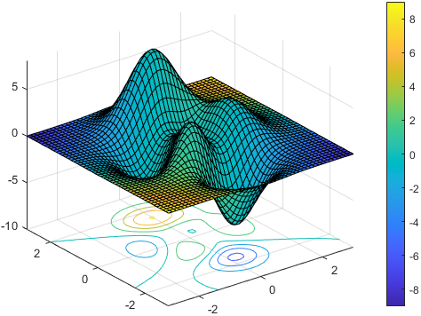
Our gradient is a vector which is a slope of the surface. As slope \( m = \frac{y}{x} \), we do the same calculation in finding the derivative. Hence It is simply a slope. So we keep finding the slope of the surface, update our values and move along the downward direction.
What after finding these gradients
As these weights and bias are initialized randomly before feedforward propagation, we update them after backpropagation.
$$ W_{\Delta} = \frac{\partial L}{\partial W_n} $$ $$ B_{\Delta} = \frac{\partial L}{\partial B_n} $$ $$ W_{new} = W_{current} - W_{\Delta} $$ $$ B_{new} = B_{current} - B_{\Delta} $$
The reason we subtract the \(W_{\Delta}\) from the current value is that we need to go to the opposite of the slope to reach global minima. Let's take an example of \(m = 2x\). \( \frac{\partial m}{\partial x} = 2 \) which is the gradient. Now increasing \(x\) by \(2\) will always increase the value of \(m\). Therefore we subtract it from the current value.
Adding Learning rate
As we saw earlier, after we find \(W_{\Delta}\) and \(B_{\Delta}\), we subtract it from \(W_{current}\) and \(B_{current}\) respectively in order to reduce the loss for next iteration. Consider that as a jump from value \(A\) to \(B\). To control the proportion of this jump, we use the learning rate. Using it, we can set how much slow or fast we want our loss to converge. So basically, the learning rate is multiplied with \( \Delta \) values as follows:
$$ W_{new} = W_{current} - ( \text{learning rate} \times W_{\Delta} ) $$ $$ B_{new} = B_{current} - ( \text{learning rate} \times B_{\Delta} ) $$
Usually we keep \(0.01\) or \(0.001\) as learning rate, but it differs on many other factors such as dataset.
steps of the neural network
iterate \(n\) times:
1. Feedforward propagation
2. Find loss between predicted images and true images
3. Backpropagation
4. Update the weights based on the gradients
Conclusion
This is all about backpropagation. While programming backpropagation, the formula is structured a bit differently in order to do mathematial operations like \( \text{dot product}\) and few others. In the upcoming posts, I will show you how to program a simple neural network from scratch and then using higher-level libraries.
Find more blogs:
Feedforward propagation - A Simple Introduction to neural networks
GUI Developement Using Python - 6. Button widget
GUI Developement Using Python - 5. Place method (Tkinter geometry Manager)
GUI Developement Using Python - 4. Grid method (Tkinter geometry manager)
GUI Developement Using Python - 3. More about Pack method (Tkinter Geometry manager)
GUI Developement Using Python - 2. Pack method (Tkinter Geometry manager)
GUI Developement Using Python - 1. Starting Tkinter
Multiple file/folder rename using Python.